Writeup for HW1: Rasterizer

This writeup is also provided on the following website: blog

Task 1: Drawing Single-Color Triangles

In this task, we implemented a simple rasterizer that draws single-color triangles on a framebuffer. The main steps involved were:

1. Defining the triangle’s bounding box.
2. Iterating over each pixel in the bounding box.
3. Checking if the pixel is inside the triangle using the edge function.
4. If the pixel is inside, we set its color in the framebuffer.

Implementation Details

• We check if a pixel is inside the triangle by checking if the point is on the same side of each edge of the triangle.
• The edge function is defined as follows:

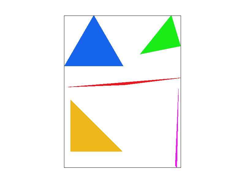
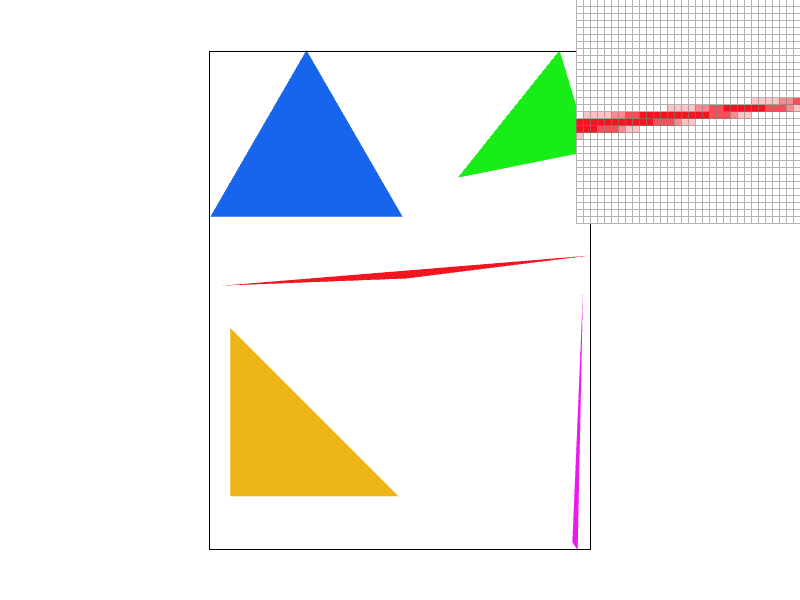
Screen shot

Extra Credit Improvements

Using the code of rasterize_line, we iterate all 3 edges, and for every possible y we calculate the x range of the triangle, so we can iterate over the x values to set the color of the pixels. This optimization reduces the number of pixel checks significantly.

Without optimize:

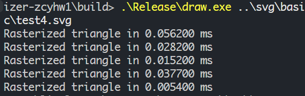
With optimize:

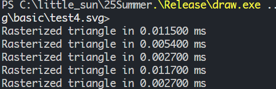
We can see that the optimized version is much faster, especially for larger triangles.

Task 2: Antialiasing by Supersampling

In this task, we implemented antialiasing for our rasterizer using supersampling. The main steps involved were:

1. For each pixel, we generate multiple sub-pixel samples.
2. We check if each sub-pixel sample is inside the triangle.
3. If a sample is inside, we accumulate its color.
4. Finally, we average the colors of all samples for each pixel.

Implementation Details

• We use a grid of samples for each pixel, where the number of samples is determined by the sample_rate.
• The fill_pixel function is modified to handle multiple samples per pixel. The color of each pixel is computed by averaging the colors of the samples that fall inside the triangle.
• We use a simple box filter for averaging the colors of the samples.

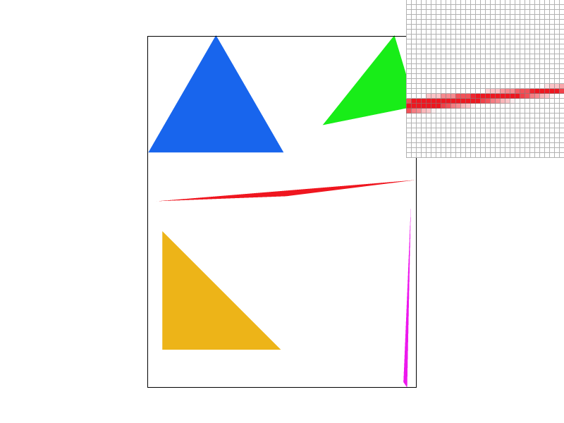
Screen shot

1 spp	4 spp	9 spp	16 spp

Extra Credit Improvements

For the extra credit, we implemented a low-discrepancy sampling method to generate the sub-pixel samples using the Halton sequence. This method ensures that the samples are evenly distributed across the pixel area, which can lead to better antialiasing results.

The Halton sequence is generated using the following function:

1
2
3
4
5
6
7
8
9
10
11
12
13
14
15
16
17
18
19
20
21
22
23

 auto radicalInverse = [](int base, int index)
{
    float result = 0.0f;
    float f = 1.0f / base;
    while (index > 0)
    {
        result += f * (index % base);
        index /= base;
        f /= base;
    }
    return result;
};
auto generateLowDiscrepancySamples = [&radicalInverse](int sampleCount,std::vector<std::pair<float, float>> &samples)
{
    samples.clear();
    for (int i = 0; i < sampleCount; ++i)
    {
        float x = radicalInverse(2, i); // base-2 for x
        float y = radicalInverse(3, i); // base-3 for y
        samples.emplace_back(x, y);
    }
};
generateLowDiscrepancySamples(sample_rate, gridDelta);

Comparison: Regular Grid vs Low-Discrepancy Sampling

Regular Grid Sampling:
| 1 spp | 4 spp | 9 spp | 16 spp |
| —————————————————————————————— | —————————————————————————————— | —————————————————————————————— | —————————————————————————————— |
| | | | |
| | | | |

The low-discrepancy sampling method using Halton sequence provides more evenly distributed samples, which can result in better antialiasing quality with reduced aliasing artifacts compared to regular grid sampling, especially in low sample rates.

Task 3: Transforms

In this task, we implemented a simple transformation system to apply translations, rotations, and scalings to triangles before rasterization. We defined transformation matrices for translation, rotation, and scaling. The matrices are:

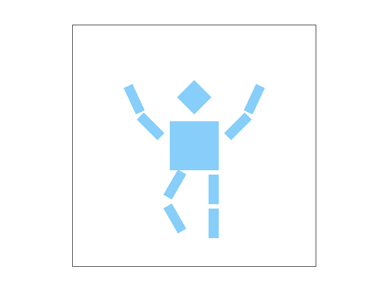
Screen shot

Here is a screenshot of my own robot, happliy waving arms and hopping around:

Task 4: Barycentric coordinates

In this task, we implemented barycentric coordinates to interpolate colors across the triangle. The barycentric coordinates are computed based on the area of the sub-triangles formed by the pixel and the triangle vertices.

Explain barycentric coordinates

Barycentric coordinates are a coordinate system used in a triangle to express the position of a point within the triangle as a weighted average of the triangle’s vertices. Given a triangle with vertices (A), (B), and (C), any point (P) inside the triangle can be represented as:

[
P = \alpha A + \beta B + \gamma C
]

where (\alpha), (\beta), and (\gamma) are the barycentric coordinates corresponding to vertices (A), (B), and (C), respectively. These coordinates have the following properties:

1. They are non-negative: (\alpha \geq 0), (\beta \geq 0), (\gamma \geq 0).
2. They sum to 1: (\alpha + \beta + \gamma = 1).

Barycentric coordinates shows the portion of each vertex’s contribution to the point (P). They are particularly useful for interpolation tasks, such as color interpolation in rasterization, as they allow for smooth transitions between vertex attributes (e.g., colors, normals) across the surface of the triangle.

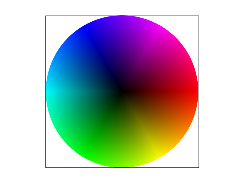
Here is an image showing how barycentric coordinates interpolate colors across a triangle:

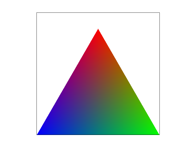
Screenshot

Here is a screenshot of the svg/basic/test7.svg with interpolated colors using barycentric coordinates:

Task 5: “Pixel sampling” for texture mapping

In this task, we implemented texture mapping using pixel sampling. The main steps involved were:

1. For each sample point, we compute the corresponding barycentric coordinates.
2. We use these coordinates to interpolate the texture coordinates from the triangle vertices.
3. Finally, we sample the texture at the interpolated texture coordinates and use the resulting color for the pixel.

Sampling Methods

We implemented two sampling methods for texture mapping:

1. Nearest Neighbor Sampling: This method samples the texture at the nearest pixel to the interpolated texture coordinates. It is simple and fast but can produce blocky artifacts.

2. Bilinear Filtering: This method samples the texture at the four nearest texels (texture pixels) and performs bilinear interpolation to compute the final color. It produces smoother results but is more computationally expensive.

Screenshot

Here is screenshots comparing the two sampling methods:

Nearest Neighbor	Bilinear Filtering

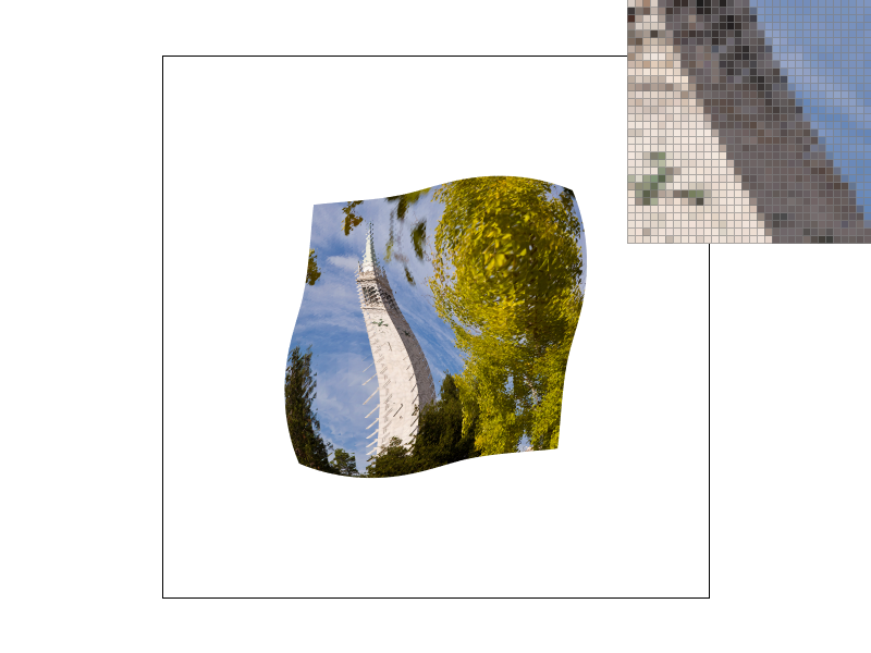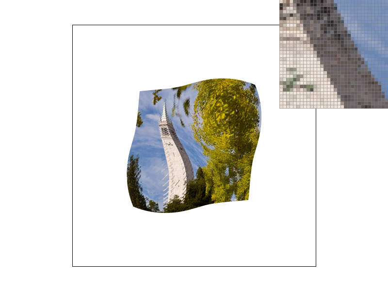As we can see, bilinear filtering produces smoother textures compared to nearest neighbor sampling, especially at lower sample rates.

The difference between nearest neighbor and bilinear filtering becomes most pronounced in the following scenarios:

1. High-frequency texture details: When the texture contains fine details or sharp transitions, nearest neighbor sampling can cause visible aliasing and pixelation, while bilinear filtering smooths these transitions.

2. Texture magnification: When the texture is being scaled up (fewer texels than screen pixels), nearest neighbor sampling results in blocky, pixelated appearance, whereas bilinear filtering creates smoother gradients between texel values.

3. Low sample rates: At 1 sample per pixel, the difference is most noticeable because there’s no additional averaging from supersampling to mask the sampling artifacts. Higher sample rates (like 16 spp) can reduce the visual difference as the supersampling provides additional smoothing.

4. Slanted or rotated textures: When texture coordinates don’t align perfectly with the texture grid, bilinear filtering provides much better results by interpolating between neighboring texels rather than snapping to the nearest one.

The fundamental reason for these differences is that nearest neighbor sampling introduces discontinuities (sudden jumps in color values), while bilinear filtering maintains continuity by smoothly interpolating between texel values, resulting in more visually pleasing and artifact-free rendering.

Task 6: “Level sampling” with mipmaps for texture mapping

As we can see, a pixel on the image may correspond to multiple texels in the texture, especially when the texture is magnified. This can lead to aliasing artifacts, where high-frequency details in the texture create visual noise or flickering.

To address this issue, we can use mipmaps, which are precomputed, downsampled versions of the original texture at different levels of detail. When rendering, we can select the appropriate mipmap level based on the screen-space size of the texture, allowing us to sample from a lower-resolution version of the texture when it is displayed at a smaller size. This helps to reduce aliasing artifacts and improve rendering performance.

Tradeoffs

When choosing between different sampling techniques, there are tradeoffs to consider:

1. Pixel Sampling (Nearest vs Bilinear)

• Speed: Nearest neighbor is fastest, bilinear requires 4 texture lookups and interpolation
• Memory: Both use same amount of memory (original texture only)
• Antialiasing: Bilinear provides better filtering of texture aliasing, nearest can be blocky

1. Level Sampling (Mipmaps)

• Speed: Faster rendering due to better cache performance with smaller textures
• Memory: Requires 33% more memory to store all mipmap levels
• Antialiasing: Excellent for reducing texture aliasing when textures are minified

1. Supersampling

• Speed: Significantly slower - O(n) where n is sample rate
• Memory: Requires n times more memory for sample buffer
• Antialiasing: Most effective against geometric aliasing (triangle edges)

Screenshot

The following screenshots show the combinations of L_ZERO and P_NEAREST, L_ZERO and P_LINEAR, L_NEAREST and P_NEAREST, as well as L_NEAREST and P_LINEAR.

	P_NEAREST	P_LINEAR
L_ZERO
L_NEAREST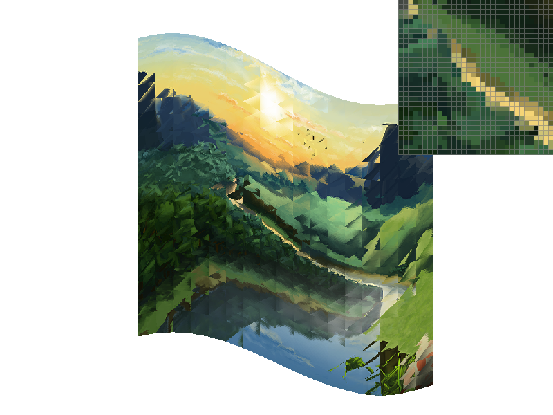

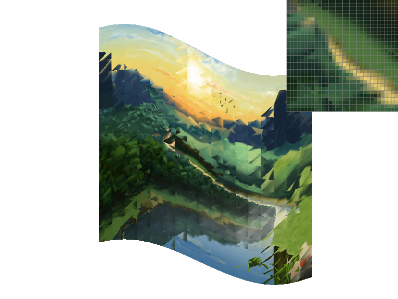Extra Credit - Draw Something Creative!

For the extra credit, I created a pattern of Nautiloidea using color interpolation.

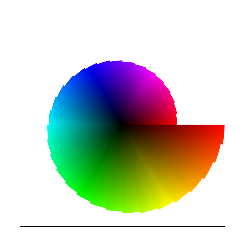
The script for generating the file is in the folder