Overview
This assignment implements a comprehensive path tracer that renders physically accurate images by simulating the behavior of light transport. The implementation progresses from basic ray tracing foundations to advanced global illumination techniques with performance optimizations.
Part 1: Ray Generation and Scene Intersection - Establishes the fundamental ray tracing pipeline, including camera ray generation, anti-aliasing through pixel sampling, and primitive intersection algorithms for triangles and spheres using mathematically robust methods like Möller-Trumbore.
Part 2: Bounding Volume Hierarchy (BVH) - Implements spatial acceleration structures to dramatically improve rendering performance. Uses axis-aligned bounding boxes and hierarchical tree traversal to reduce intersection tests from O(n) to O(log n) complexity.
Part 3: Direct Illumination - Develops realistic lighting models through Bidirectional Scattering Distribution Functions (BSDFs) and Monte Carlo integration. Compares uniform hemisphere sampling against importance sampling techniques to achieve variance reduction and noise-free rendering.
Part 4: Global Illumination - Extends to full light transport simulation with recursive path tracing, implementing multi-bounce lighting effects, Russian Roulette optimization for unbiased path termination, and comprehensive analysis of direct vs. indirect illumination contributions.
Part 5: Adaptive Sampling - Introduces intelligent sampling optimization that concentrates computational effort where needed most. Uses statistical convergence analysis with 95% confidence intervals to achieve superior image quality with fewer samples through selective pixel-level adaptation.
AI acknowledgements
This assignment was completed with assistance from GitHub Copilot (GPT-4), which provided:
Code implementation guidance: Assistance with implementing small code snippets, while the main algorithmic structure and logic were designed and coded by myself.
Mathematical formulation: I use the AI to help clarify mathematical concepts and equations related to ray tracing, BVH construction, and Monte Carlo integration.
Documentation and analysis: Same as above, the AI helped me to deeply understand the concepts, thus I could write the explanations and analyses in the writeup.
Debugging and optimization: AI Assisted me with identifying and resolving implementation issues, particularly in complex areas like BVH construction and traversal.
All fundamental concepts, algorithmic understanding, and final implementation decisions were made by myself. The AI served as a coding assistant and conceptual guide, but the core intellectual work and design were my own.
Part 1: Ray Generation and Scene Intersection
Ray Generation and Primitive Intersection Pipeline
The rendering pipeline for ray generation and primitive intersection consists of several key stages that work together to determine what objects are visible at each pixel:
1. Pixel Sampling Stage (PathTracer::raytrace_pixel)
For each pixel in the image:
- Input: Pixel coordinates $(x, y)$ in image space, where $(0,0)$ is at the bottom-left corner
- Anti-aliasing: Generate multiple sample points within the pixel using a grid sampler
- Coordinate transformation: Convert pixel coordinates to normalized coordinates $[0,1] \times [0,1]$ for the camera
- Sample accumulation: Average the radiance values from all samples within the pixel
The implementation generates ns_aa random samples within each pixel to reduce aliasing artifacts. Each sample point is obtained using gridSampler->get_sample() which provides uniform random samples in the unit square $[0,1) \times [0,1)$.
2. Camera Ray Generation Stage (Camera::generate_ray)
For each sample point:
- Input: Normalized image coordinates $(x, y) \in [0,1] \times [0,1]$
- Camera space transformation: Map image coordinates to the virtual sensor plane at $z = -1$
- Ray direction calculation: Compute ray direction from camera origin through the sensor point
- World space transformation: Transform the ray from camera space to world space using the camera-to-world matrix
- Output: A ray with proper origin, direction, and clipping planes
The camera space coordinate system has:
- Camera positioned at origin $(0,0,0)$
- Viewing direction along $-Z$ axis
- Sensor plane at $z = -1$
- Sensor bounds: bottom-left at $(-\tan(\frac{hFov}{2}), -\tan(\frac{vFov}{2}), -1)$ and top-right at $(\tan(\frac{hFov}{2}), \tan(\frac{vFov}{2}), -1)$
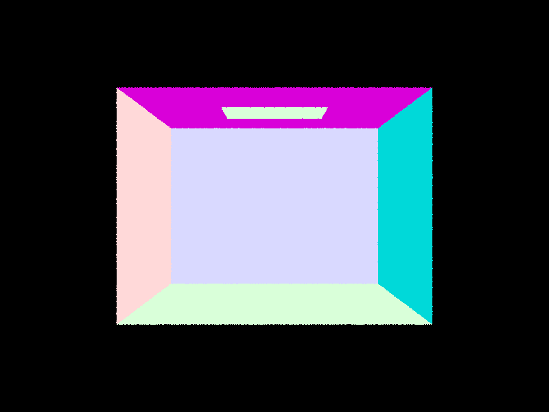
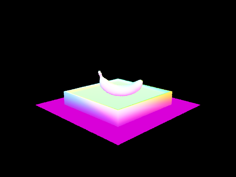
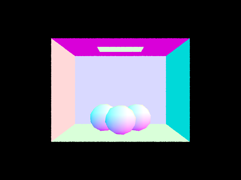
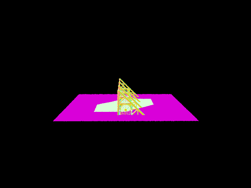
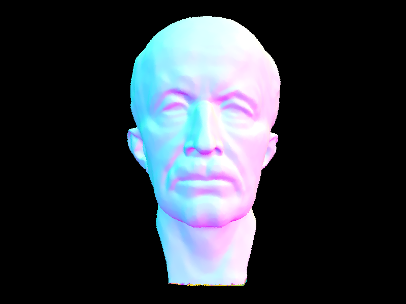
After generating the ray, the results of rendering sky/CBempty.dae and keenan/banana.dae is shown in the provided images.

3. Primitive Intersection Stage
The primitive intersection normally have these stages:
- Ray Generation
Generate rays from the camera (or light) into the scene—each ray corresponds to a pixel (or a light sample). - Acceleration‐Structure Traversal
Walk a spatial index (e.g. BVH/KD‑Tree) to quickly cull away large chunks of geometry that the ray cannot hit. - Primitive Intersection Test
For the handful of remaining triangles (or other primitives), run a fast per‐primitive test (e.g. Möller–Trumbore) to compute if—and where—the ray intersects. - Closest‐Hit Selection
Keep only the intersection with the smallest positive distance along the ray, discarding all others.
This stage determines where a ray actually meets the scene geometry (if at all) and gathers the hit’s position, surface normal, UVs, etc. Those data are essential inputs for shading, shadow checks, reflections/refractions, and ultimately for computing the final color of each pixel.
Primitive Intersection Details
Triangle Intersection Algorithm (Möller-Trumbore):
The triangle intersection implementation uses the Möller-Trumbore algorithm, which is an efficient method for computing ray-triangle intersections. Here’s how it works:
- Setup: Given a triangle with vertices $\mathbf{p_1}, \mathbf{p_2}, \mathbf{p_3}$ and a ray with origin $\mathbf{O}$ and direction $\mathbf{D}$
- Edge vectors: Compute $\mathbf{e_1} = \mathbf{p_2} - \mathbf{p_1}$ and $\mathbf{e_2} = \mathbf{p_3} - \mathbf{p_1}$
- Determinant check: Calculate $\mathbf{h} = \mathbf{D} \times \mathbf{e_2}$ and $a = \mathbf{e_1} \cdot \mathbf{h}$
- If $|a| < \epsilon$, the ray is parallel to the triangle (no intersection)
- Barycentric coordinate u: Compute $\mathbf{s} = \mathbf{O} - \mathbf{p_1}$ and $u = \dfrac{\mathbf{s} \cdot \mathbf{h}}{a}$
- If $u < 0$ or $u > 1$, the intersection point is outside the triangle
- Barycentric coordinate v: Compute $\mathbf{q} = \mathbf{s} \times \mathbf{e_1}$ and $v = \dfrac{\mathbf{D} \cdot \mathbf{q}}{a}$
- If $v < 0$ or $u + v > 1$, the intersection point is outside the triangle
- Parameter t: Calculate $t = \dfrac{\mathbf{e_2} \cdot \mathbf{q}}{a}$
- If $t \in [t_{min}, t_{max}]$, we have a valid intersection
The algorithm provides barycentric coordinates $(u, v, w)$ where $w = 1 - u - v$, which are used to interpolate vertex normals:
- Interpolated normal = $w \cdot \mathbf{n_1} + u \cdot \mathbf{n_2} + v \cdot \mathbf{n_3}$
This method is both numerically stable and efficient, avoiding the need to compute the plane equation explicitly.
Sphere Intersection:
For ray-sphere intersection, we solve a quadratic equation. Given a sphere with center $\mathbf{C}$ and radius $r$, and a ray $\mathbf{R}(t) = \mathbf{O} + t\mathbf{D}$
The intersection occurs when $|\mathbf{R}(t) - \mathbf{C}|^2 = r^2$, which expands to:
This gives us the quadratic equation:
where:
- $a = \mathbf{D} \cdot \mathbf{D}$
- $b = 2\mathbf{D} \cdot (\mathbf{O} - \mathbf{C})$
- $c = |\mathbf{O} - \mathbf{C}|^2 - r^2$
The algorithm:
- Computes the discriminant $\Delta = b^2 - 4ac$
- If $\Delta < 0$, no intersection exists
- Otherwise, solves for $t = \dfrac{-b \pm \sqrt{\Delta}}{2a}$
- Chooses the smaller positive $t$ value within $[t_{min}, t_{max}]$
- Computes surface normal as $\mathbf{n} = \dfrac{\mathbf{R}(t) - \mathbf{C}}{r}$
Task 1: Generating Camera Rays
The camera ray generation transforms normalized screen coordinates to world-space rays through the camera’s virtual sensor plane.
Task 2: Generating Pixel Samples
The pixel sampling averaging multiple random samples within each pixel for anti-aliasing.
Task 3: Ray-Triangle Intersection
The ray-triangle intersection uses the Möller-Trumbore algorithm for efficient and robust intersection testing. After implementing this task, rendering sky/CBempty.dae produces normal-shaded geometry:
Task 4: Ray-Sphere Intersection
The ray-sphere intersection implements the quadratic equation method described earlier. The implementation includes three functions:
test(): Core intersection algorithm that solves the quadratic equation and returns both intersection parameters $t_1$ and $t_2$has_intersection(): Quick intersection test that checks if any valid intersection exists within the ray’s range and updatesmax_tintersect(): Complete intersection that computes intersection data and updates the ray’smax_t
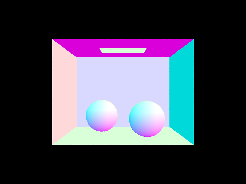
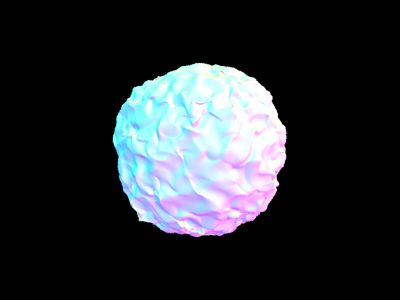
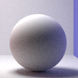
After implementing this task, rendering sky/CBspheres_lambertian.dae produces sphere geometry with normal shading:
Some more screenshots
Part 2: Bounding Volume Hierarchy
Task 1: BVH Construction
The Bounding Volume Hierarchy (BVH) is a tree data structure that hierarchically organizes geometric primitives to accelerate ray-primitive intersection tests. Our implementation uses the axis midpoint heuristic for constructing the BVH.
Algorithm Overview
The BVH construction algorithm works recursively:
- Base Case: If the number of primitives ≤
max_leaf_size, create a leaf node - Recursive Case:
- Choose the longest axis of the bounding box
- Split primitives at the midpoint of that axis
- Recursively build left and right subtrees
BVH Construction Mathematics
For a bounding box with extent $\mathbf{e} = (e_x, e_y, e_z)$, we choose the split axis as:
The midpoint along the chosen axis is:
Each primitive is assigned to the left or right subtree based on its centroid:
Where primitive $i$ goes to the left subtree if $\text{centroid}_i[\text{split_axis}] < \text{midpoint}$.
Edge Case Handling
To prevent degenerate splits where all primitives end up on one side, we implement a fallback mechanism that ensures both subtrees have at least one primitive by splitting at the median position when the midpoint heuristic fails.
Task 2: Bounding Box Intersection
For efficient BVH traversal, we need to implement ray-bounding box intersection. An axis-aligned bounding box (AABB) can be viewed as the intersection of three slabs, where each slab is defined by two parallel planes perpendicular to a coordinate axis.
Mathematical Foundation
For each axis $i \in \{x, y, z\}$, the bounding box is bounded by planes at coordinates $\text{min}_i$ and $\text{max}_i$. A ray $\mathbf{r}(t) = \mathbf{o} + t\mathbf{d}$ intersects these planes at times:
where $\mathbf{o}$ is the ray origin and $\mathbf{d}$ is the ray direction.
Algorithm Implementation
- Initialize intervals: Start with the input time interval $[t_0, t_1]$
- Process each axis: For each coordinate axis $i$:
- If $|d_i| < \epsilon$ (ray parallel to slab):
- Check if $o_i \in [\text{min}_i, \text{max}_i]$
- If outside, return false (no intersection)
- Otherwise:
- Compute $t_{\text{near}}^{(i)}$ and $t_{\text{far}}^{(i)}$
- Ensure $t_{\text{near}}^{(i)} \leq t_{\text{far}}^{(i)}$ (swap if necessary)
- Update interval: $t_{\text{min}} = \max(t_{\text{min}}, t_{\text{near}}^{(i)})$, $t_{\text{max}} = \min(t_{\text{max}}, t_{\text{far}}^{(i)})$
- Early exit if $t_{\text{min}} > t_{\text{max}}$ (empty intersection)
- If $|d_i| < \epsilon$ (ray parallel to slab):
- Final intersection: The ray intersects the box in interval $[t_{\text{min}}, t_{\text{max}}]$
The final intersection interval is:
This method is highly efficient with $O(1)$ complexity and handles all edge cases including parallel rays and negative ray directions.
Task 2.3: BVH Traversal
With bounding box intersection implemented, we can now perform efficient BVH traversal. The BVH acceleration structure uses recursive traversal to quickly eliminate large portions of the scene that don’t intersect with a ray.
Algorithm Overview
The BVH traversal algorithm works as follows:
- Bounding Box Test: First test if the ray intersects the current node’s bounding box
- Leaf Node Processing: If it’s a leaf node, test intersection with all primitives in the node
- Internal Node Processing: If it’s an internal node, recursively traverse both children
Implementation Details
has_intersection() function:
- Provides early termination optimization - returns
trueas soon as any intersection is found - Used for shadow ray testing where we only need to know if there’s any blocker
- Updates intersection statistics but doesn’t need to find the closest hit
intersect() function:
- Must find the closest intersection along the ray
- Updates the ray’s
max_tparameter to ensure subsequent tests only consider nearer intersections - Returns complete intersection information including surface normal, UV coordinates, and material
BVH Traversal Efficiency
For a ray $\mathbf{r}(t) = \mathbf{o} + t\mathbf{d}$, the BVH traversal maintains the invariant that any intersection at parameter $t’$ satisfies $t_{\text{min}} \leq t’ \leq t_{\text{max}}$ where $[t_{\text{min}}, t_{\text{max}}]$ is the current search interval.
The algorithm’s efficiency comes from the hierarchical culling:
- If a ray doesn’t intersect a node’s bounding box, it cannot intersect any primitives within that subtree
- This provides $O(\log n)$ expected complexity instead of $O(n)$ for naive intersection testing
Time Comparison
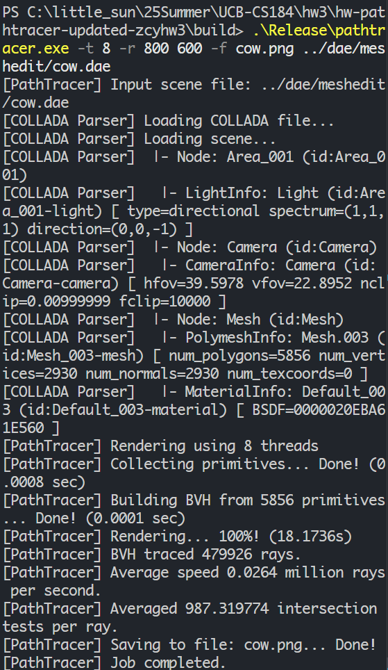
To evaluate the performance of the ray tracer with and without a bounding volume hierarchy (BVH), we conducted timing experiments on scenes with varying complexity.
The cow scene rendered without BVH took approximately 18 seconds:
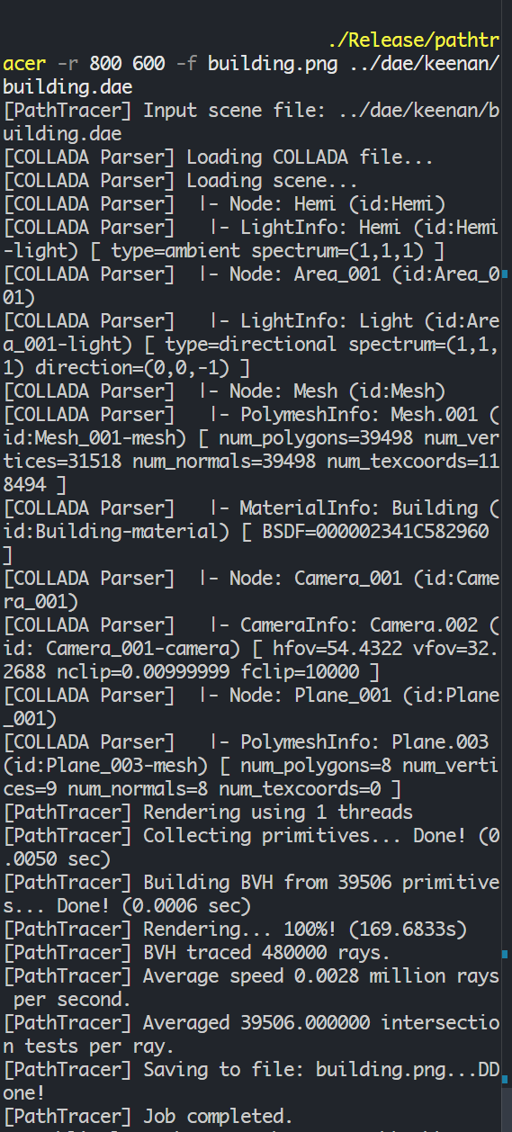
The keenan/building.dae scene rendered without BVH took approximately 170 seconds:
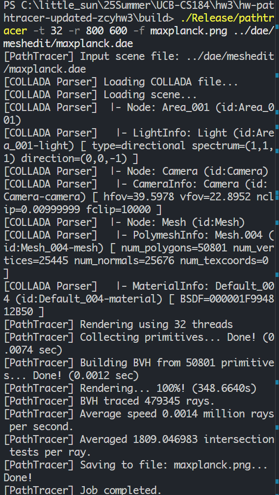
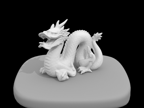
The meshedit/maxplanck.dae scene rendered without BVH took approximately 350 seconds:
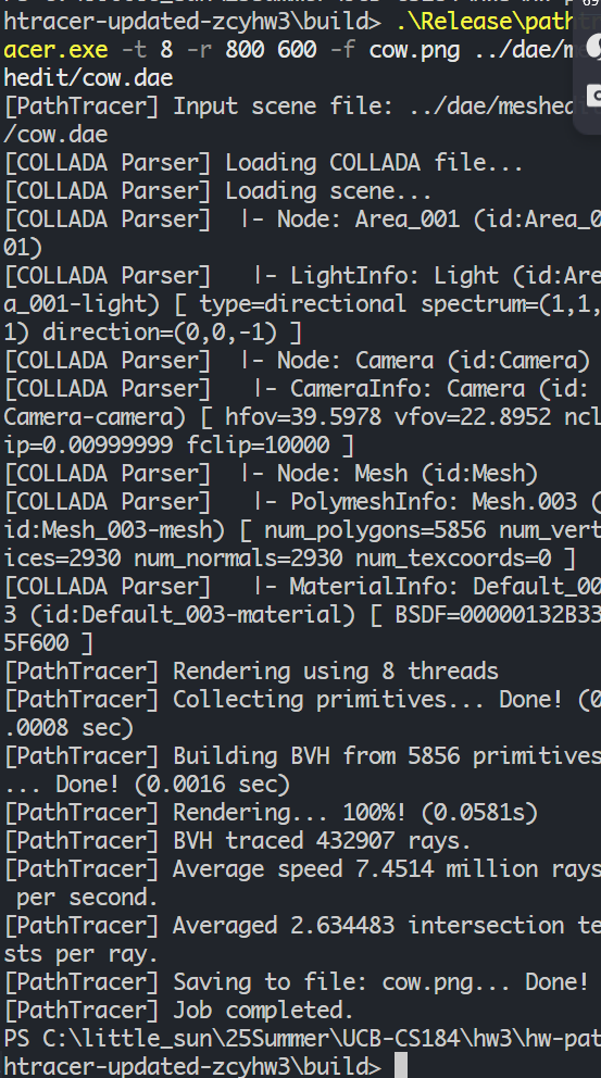
Rendering the cow scene with BVH took approximately 0.05 seconds:
Rendering the building scene with BVH took approximately 0.1 seconds: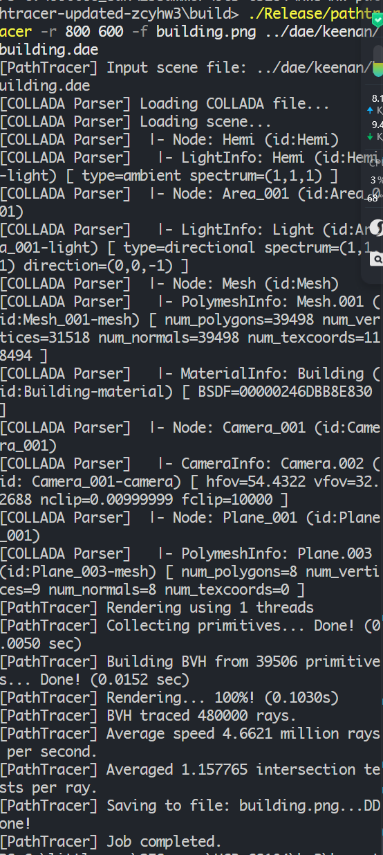
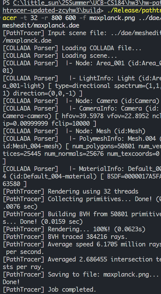
Rendering the Max Planck scene with BVH took approximately 0.06 seconds:
As the result shown, the BVH significantly accelerates ray-primitive intersection tests, reducing rendering times from minutes to fractions of a second for complex scenes. This demonstrates the effectiveness of spatial acceleration structures in ray tracing.
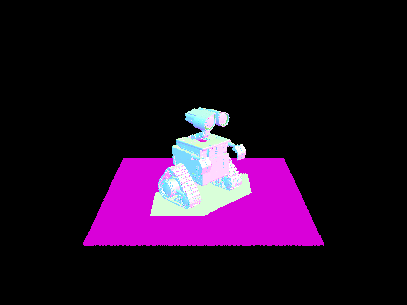
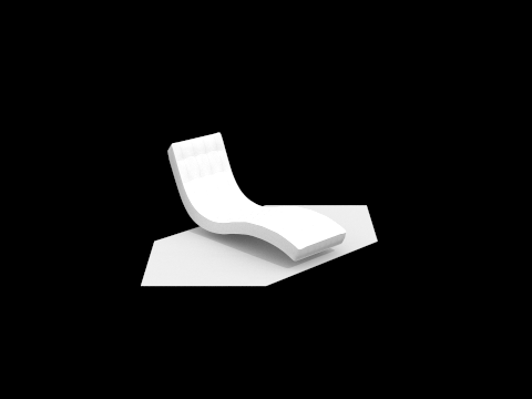
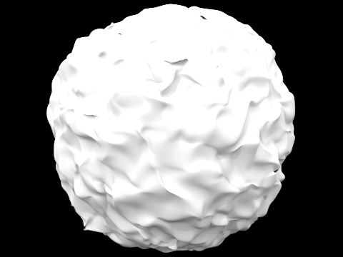
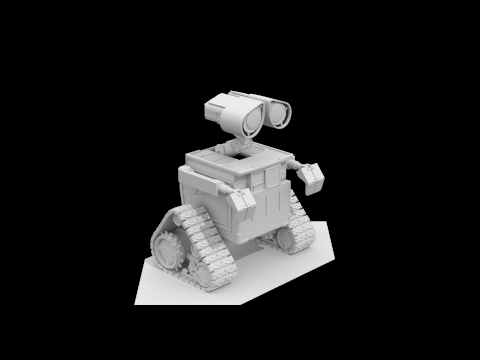
Results showcase

Part 3: Direct Illumination
Task 1: Diffuse BSDF
The Bidirectional Scattering Distribution Function (BSDF) describes how light interacts with surfaces. For diffuse materials, we implement the Lambertian reflection model, which assumes that reflected light is scattered uniformly in all directions according to Lambert’s cosine law.
BSDF Mathematical Model
For a Lambertian surface, the BSDF is constant for all outgoing directions and is given by:
where:
- $\rho$ is the reflectance (albedo) of the surface, representing the fraction of incident light that is reflected
- $\pi$ is the normalization factor ensuring energy conservation
- $\omega_o$ is the outgoing (viewing) direction
- $\omega_i$ is the incoming (light) direction
BSDF Implementation
f() function:
Returns the BSDF value for any pair of incident and outgoing directions. For diffuse materials, this is simply reflectance / π.
Cosine-Weighted Sampling
The cosine-weighted hemisphere sampler generates directions according to the distribution:
where $\theta$ is the angle between the sampled direction and the surface normal. This distribution naturally accounts for Lambert’s cosine law, making it an efficient sampling strategy for diffuse materials.
Task 2: Zero-bounce Illumination
The zero-bounce illumination function computes the emitted light from surfaces that are directly visible to the camera without any bounces. This is particularly important for emissive materials, such as light sources.
The implementation simply returns isect.bsdf->get_emission(), which represents the intrinsic light emission of the intersected surface.
Task 3: Direct Lighting with Uniform Hemisphere Sampling
This task implements direct illumination using Monte Carlo integration with uniform hemisphere sampling. The goal is to estimate how much light arrives at a surface point from all directions in the hemisphere above the surface.
Direct Lighting Algorithm
The direct lighting estimation follows these steps:
- Hemisphere Sampling: For each sample, use
UniformHemisphereSampler3D::get_sample()to generate a random direction in the local coordinate system - World Space Transformation: Transform the sampled direction from object space to world space using the
o2wmatrix - Shadow Ray Casting: Create a shadow ray from the hit point in the sampled direction with
min_t = EPS_Fto avoid self-intersection - Light Source Detection: Check if the shadow ray intersects a light source by testing if
emission.norm() > 0 - BSDF Evaluation: Compute the BSDF value using
isect.bsdf->f(w_out, w_in_local) - Monte Carlo Integration: Apply the reflection equation with proper normalization
Hemisphere Sampling Mathematics
The Monte Carlo estimator for the reflection equation is:
For uniform hemisphere sampling:
- Probability density function: $p(\omega) = \frac{1}{2\pi}$
- Cosine term: $\cos\theta_i = \omega_i \cdot \mathbf{n} = w_{i,z}$ (in local coordinates where normal is $(0,0,1)$)
Task 4: Direct Lighting by Importance Sampling Lights
While hemisphere sampling works correctly, it can be quite noisy and inefficient. Importance sampling directly samples the light sources instead of random hemisphere directions, which significantly reduces variance and enables rendering of point light sources.
Importance Sampling Strategy
Instead of sampling random directions and hoping to hit light sources, importance sampling works by:
- Light Source Iteration: Loop through each light in the scene
- Light Sampling: For each light, use
SceneLight::sample_L()to generate samples pointing toward the light - Shadow Ray Testing: Cast shadow rays to check for occlusion between the surface and light
- BSDF Evaluation: Apply the reflection equation using the light samples
Light Sampling Implementation
Point Light Optimization:
- Point lights (
is_delta_light() == true) only need one sample since all samples produce identical results - Area lights require multiple samples (
ns_area_light) to capture the light’s spatial extent
Shadow Ray Setup:
- Origin: Surface hit point with
min_t = EPS_Foffset - Direction: Toward the light source (from
sample_L) - Max distance:
distToLight - EPS_Fto avoid intersecting the light itself - Occlusion test: If shadow ray intersects any geometry, the point is in shadow
Importance Sampling Mathematics
The importance sampling estimator becomes:
where:
- $N_{\text{light}}$ is the number of samples per light source
- $p_{\text{light}}(\omega_i)$ is the probability density function provided by the light source
- $V(p, \omega_i)$ is the visibility function (1 if unoccluded, 0 if in shadow)
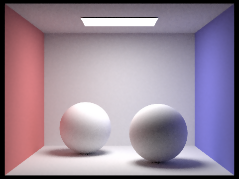
Image Comparison
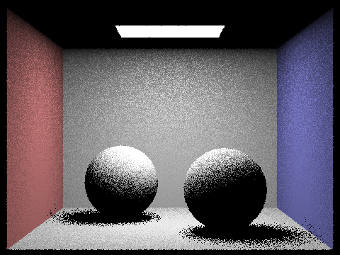
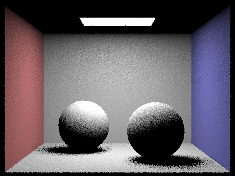
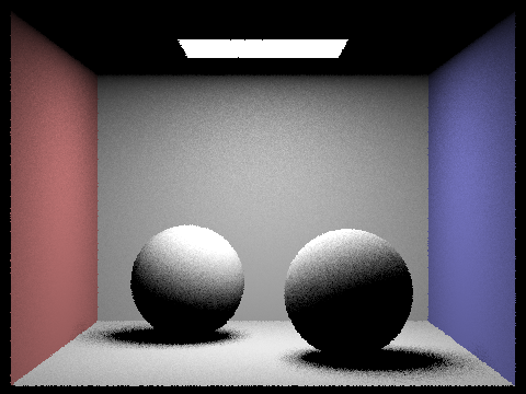
To compare the results of uniform hemisphere sampling and importance sampling, we rendered the same scene using both methods. The images below illustrate the difference in noise levels and convergence speed.

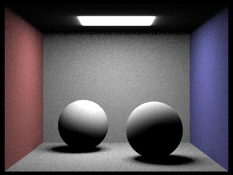

The following image sequence demonstrates how increasing light ray count (-l flag) progressively reduces noise in soft shadow regions. Higher light ray counts produce smoother, more natural-looking shadows with less noise, while lower counts result in speckled, grainy shadow boundaries. This occurs because soft shadows are created by area lights, and more light samples better capture the partial occlusion effects across the light’s spatial extent, reducing Monte Carlo variance.

Analysis: Hemisphere Sampling vs. Importance Sampling
The comparison between uniform hemisphere sampling and importance sampling reveals significant differences in both image quality and computational efficiency. Hemisphere sampling produces noticeably noisier images, particularly in shadow regions and areas with indirect lighting, due to the many wasted samples that don’t contribute to illumination when random directions fail to hit light sources. In contrast, importance sampling generates much cleaner images with smoother gradients and more accurate shadow boundaries by directly sampling light sources, ensuring that every sample contributes meaningful illumination information. The noise reduction is especially pronounced in soft shadow regions where hemisphere sampling struggles with variance, while importance sampling’s direct light-to-surface sampling provides consistent, low-variance estimates. Additionally, importance sampling enables rendering of point light sources, which hemisphere sampling cannot handle effectively since the probability of randomly hitting a zero-area point light is negligible. Overall, importance sampling achieves superior image quality with fewer samples, demonstrating the critical role of variance reduction techniques in Monte Carlo rendering and making it the preferred method for direct illumination in production ray tracers.
Part 4: Global Illumination
Task 1: Sampling with Diffuse BSDF
sample_f() function:
- Samples an outgoing direction $\omega_i$ using cosine-weighted hemisphere sampling
- Returns the BSDF evaluation for the sampled direction
- Updates the probability density function (PDF) for importance sampling
Task 2: Global Illumination with up to N Bounces of Light
The global illumination implementation extends direct lighting to include indirect lighting through multiple light bounces. This creates realistic color bleeding, soft shadows, and ambient lighting effects that make rendered images more visually convincing.
Implementation Overview
The core function at_least_one_bounce_radiance() implements recursive path tracing to calculate both direct and indirect illumination. The algorithm follows these key steps:
- Direct Lighting Calculation: Always include one-bounce (direct) lighting from light sources
- BSDF Sampling: Sample outgoing directions using the material’s BSDF for importance sampling
- Recursive Ray Tracing: Cast secondary rays and recursively calculate lighting
- Monte Carlo Integration: Apply the rendering equation with proper normalization
Rendering Equation Foundation
The rendering equation for global illumination is:
Where:
- $L_o(p, \omega_o)$ is the outgoing radiance at point $p$ in direction $\omega_o$
- $L_e(p, \omega_o)$ is the emitted radiance (handled by
zero_bounce_radiance) - $f_r(p, \omega_i, \omega_o)$ is the BSDF value
- $L_i(p, \omega_i)$ is the incoming radiance (calculated recursively)
- $\cos\theta_i$ is the cosine of the angle between incident direction and surface normal
Detailed Algorithm Implementation
Accumulation Mode Handling:
The implementation supports two modes controlled by the isAccumBounces parameter:
Accumulation Mode (
isAccumBounces = true):- Accumulates all bounces from 1 to
max_ray_depth - Always includes direct lighting
- Recursively adds all indirect contributions
- Accumulates all bounces from 1 to
Specific Bounce Mode (
isAccumBounces = false):- Returns only the light from the
max_ray_depth-th bounce - Traces through intermediate bounces without accumulating them
- Used for analyzing individual bounce contributions
- Returns only the light from the
1 | if (isAccumBounces) |
Indirect Lighting Calculation:
For each intersection point, the algorithm samples the BSDF to determine the next ray direction:
1 | Vector3D w_in; |
The sample_f function uses cosine-weighted hemisphere sampling for diffuse materials, which provides importance sampling that naturally accounts for Lambert’s cosine law.
Ray Continuation:
1 | Vector3D w_in_world = o2w * w_in; // Transform to world coordinates |
Recursive Integration:
The Monte Carlo estimator for the rendering equation becomes:
Where $p(\omega_i)$ is the probability density function from BSDF sampling.
1 | if (bvh->intersect(new_ray, &new_isect)) |
Task 3: Global Illumination with Russian Roulette
To optimize the path tracing process and reduce computation time, we implement Russian Roulette to probabilistically terminate light paths.
Russian Roulette is a variance reduction technique that randomly terminates ray paths while maintaining an unbiased Monte Carlo estimator. Instead of always tracing rays to a fixed maximum depth, we probabilistically decide whether to continue or terminate each path based on a continuation probability.
Implementation Process
The Russian Roulette implementation follows these key steps:
Termination Probability: We use a termination probability of
0.35, meaning there’s a 35% chance to terminate the path at each bounce (continuation probability = 0.65)Random Decision: At each bounce level (when
r.depth > 1), we use thecoin_flip(termination_prob)function to randomly decide whether to terminate the pathUnbiased Compensation: When we continue tracing (path not terminated), we scale the contribution by
1/continuation_probto maintain an unbiased estimator
Mathematical Foundation
For an unbiased estimator, when we terminate with probability $p$ and continue with probability $(1-p)$, the contribution must be scaled by $\dfrac{1}{1-p}$ when the path continues:
This maintains the correct expected radiance while reducing computational cost by terminating some paths early.
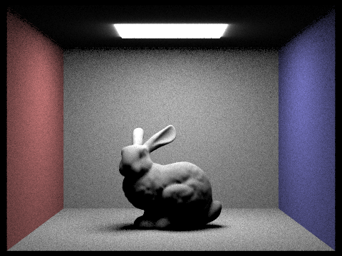
Global Illumination Results
Here are some results showcasing the effects of global illumination.


Direct / Indirect Illumination Comparison
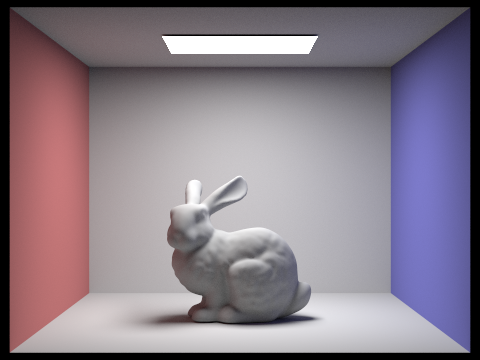
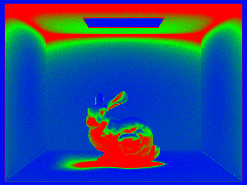
The following images demonstrate the difference between direct illumination only and indirect illumination only for CBbunny.dae using 1024 samples per pixel:
| Direct Illumination Only (m=1) | Indirect Illumination Only (m=5) | |
|---|---|---|
| CBbunny | 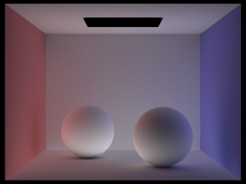 |
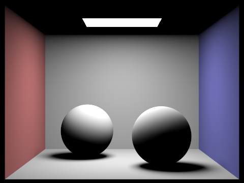 |
Direct illumination shows only the light that arrives directly from light sources to surfaces, creating sharp shadows and clear lighting boundaries. Indirect illumination captures the subtle color bleeding, soft ambient lighting, and inter-reflections that occur when light bounces between surfaces, filling in the harsh shadows with realistic ambient lighting effects.
Accumulated and Unaccumulated CBBunny
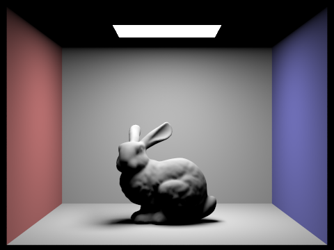
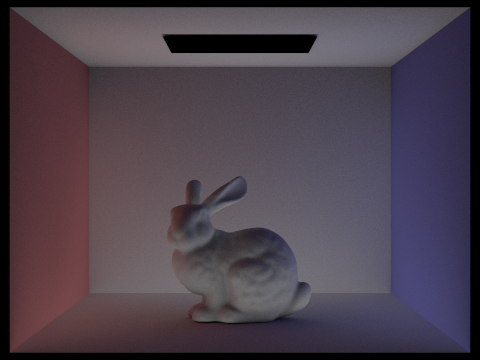
The following images compare accumulated vs unaccumulated bounces for CBbunny.dae with different max ray depths using 1024 samples per pixel.
Accumulated Bounces (isAccumBounces=true)
| Max Ray Depth 0 | Max Ray Depth 1 | Max Ray Depth 2 | |
|---|---|---|---|
| Image |  |
 |
 |
| Max Ray Depth 3 | Max Ray Depth 4 | Max Ray Depth 5 | |
|---|---|---|---|
| Image | 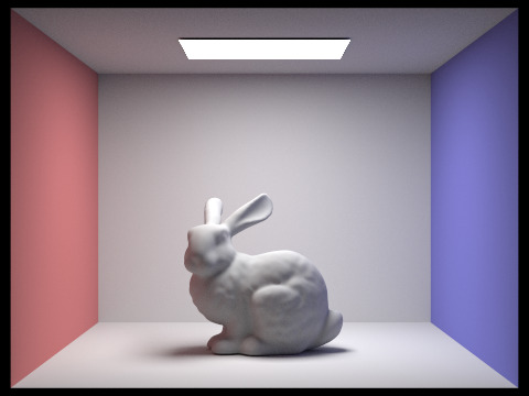 |
 |
|
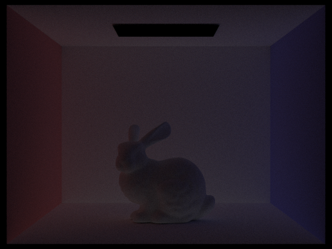
Unaccumulated Bounces (isAccumBounces=false)
| Max Ray Depth 0 | Max Ray Depth 1 | Max Ray Depth 2 | |
|---|---|---|---|
| Image |  |
 |
 |
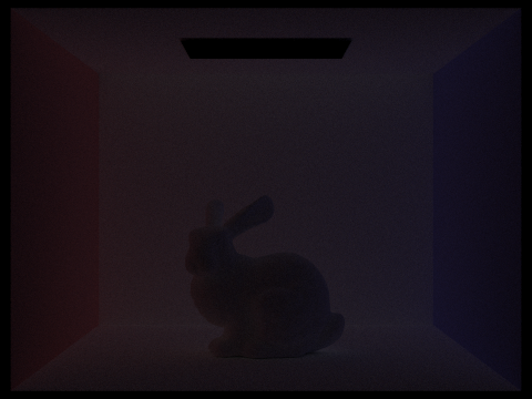
| Max Ray Depth 3 | Max Ray Depth 4 | Max Ray Depth 5 | |
|---|---|---|---|
| Image | 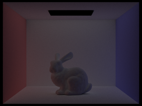 |
 |
 |
‣ 2‑bounce image (one indirect bounce)
- Scene is still fairly bright because light has only scattered once after the first surface hit.
- Clear red bleed on the left and blue bleed on the right where wall colours are reflected onto the bunny and floor.
- Shadows already soften; large dark areas are replaced by gentle gradients.
‣ 3‑bounce image (two indirect bounces)
- Overall luminance drops sharply.
- Colour bleeding is still present but subtler; instead you notice a faint “fill light” in recesses and room corners that were darker in the 2‑bounce image.
- Looks a bit noisier because far fewer sampled paths survive.
VS. rasterization
Rasterization normally captures direct light only; any global‑illumination effects (colour bleeding, soft indirect shadows, corner darkening) must be faked with ambient terms, SSAO, light‑maps, etc. In contrast, Path tracing’s extra bounces physically simulate those effects:
| Effect | Achieved by 2nd bounce | Refined by 3rd‑plus bounces | Rasterization counterpart |
|---|---|---|---|
| Colour bleeding | Provides the majority of visible tinting | Adds faint, wider‑area tints | Requires baked light‑maps or screen‑space GI |
| Soft shadow penumbrae | Already visible | Further smooths deep crevices | Shadow‑maps + blur |
| Ambient fill / corner fall‑off | Begins to appear | Removes last unrealistically black pockets | Ambient term / SSAO |
Thus, each additional bounce brings the rendered frame closer to a physically correct global‑illumination solution.
Russian Roulette CBBunny
The following images demonstrate different max ray depths with Russian Roulette enabled on rendering quality and performance. Use 1024 samples per pixel.
| Max Ray Depth 0 | Max Ray Depth 1 | Max Ray Depth 2 | |
|---|---|---|---|
| Image |  |
 |
 |
| Max Ray Depth 3 | Max Ray Depth 4 | Max Ray Depth 100 | |
|---|---|---|---|
| Image |  |
 |
 |
The key benefit of Russian Roulette is that it allows for potentially infinite bounces while maintaining finite expected computation time. The termination probability of 0.35 provides a good balance between performance and quality.
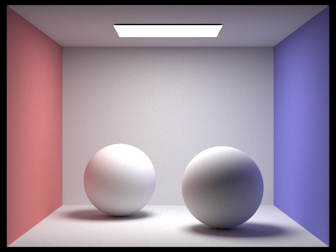
Various spp Showcase
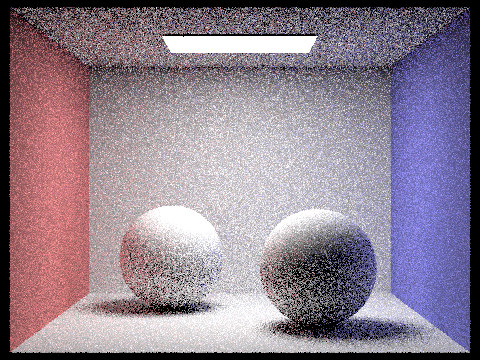
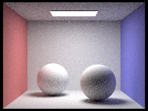
The following images demonstrate the effect of different sample-per-pixel rates on rendering quality for CBspheres scene. Use 4 light rays.
| 1 spp | 2 spp | 4 spp | 8 spp | |
|---|---|---|---|---|
| Image | 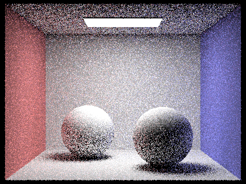 |
 |
 |
 |
| 16 spp | 64 spp | 1024 spp | |
|---|---|---|---|
| Image |  |
 |
|
Part 5: Adaptive Sampling
Adaptive Sampling Overview
Adaptive sampling is an optimization technique that concentrates computational effort where it’s needed most, rather than using a fixed number of samples per pixel uniformly across the entire image. Some pixels converge to a stable color value with relatively few samples, while others require many more samples to eliminate noise effectively.
Adaptive Sampling Algorithm
The adaptive sampling algorithm works by monitoring the convergence of each pixel individually using statistical analysis. For each pixel, we track two running statistics:
- $s_1 = \sum_{k=1}^{n} x_k$ (sum of illuminance values)
- $s_2 = \sum_{k=1}^{n} x_k^2$ (sum of squared illuminance values)
Where $x_k$ is the illuminance of the $k$-th sample, calculated using Vector3D::illum().
From these statistics, we compute the mean and variance:
- Mean: $\mu = \frac{s_1}{n}$
- Variance: $\sigma^2 = \frac{1}{n-1} \cdot \left(s_2 - \frac{s_1^2}{n}\right)$
The convergence measure is defined as:
This represents a 95% confidence interval for the pixel’s true average illuminance. The pixel is considered converged when:
Adaptive Sampling Implementation
- Sample Generation: Generate camera rays and estimate radiance as usual
- Statistics Tracking: For each sample, update $s_1$ and $s_2$ with the sample’s illuminance
- Batch Processing: Check convergence every
samplesPerBatchsamples to avoid excessive computation - Convergence Testing: Calculate $I$ and compare against the tolerance threshold
- Early Termination: Stop sampling if the pixel converges before reaching maximum samples
- Sample Count Recording: Update
sampleCountBufferwith the actual number of samples used
Adaptive Sampling Results
The following images demonstrate adaptive sampling with different scenes and parameters:
CBbunny Scene - Adaptive Sampling
| Rendered Image | Sampling Rate Image |
|---|---|
 |
 |
Parameters: 2048 max samples, batch size = 64, tolerance = 0.05, 1 sample per light, max ray depth = 5
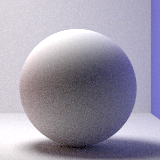
CBspheres Scene - Adaptive Sampling
| Rendered Image | Sampling Rate Image |
|---|---|
 |
 |
Parameters: 2048 max samples, batch size = 64, tolerance = 0.05, 1 sample per light, max ray depth = 5
Extra Credit
Part 1: Low Discrepancy Sampling
Low discrepancy sampling, such as Halton or Hammersley sequences, provides more uniform coverage of the sample space compared to purely random sampling, leading to faster convergence and reduced noise in Monte Carlo integration.
Low Discrepancy Algorithm
The low discrepancy sampler uses the Halton sequence with prime bases 2 and 3 for generating 2D samples:
- Base 2 (x-coordinate): Provides binary digit reversal sequence
- Base 3 (y-coordinate): Provides ternary digit reversal sequence
- Sample generation:
(halton(i, 2), halton(i, 3))for the i-th sample
The Halton sequence ensures better stratification across the unit square compared to random sampling.
Comparison Results
The following images compare uniform random sampling vs. low discrepancy sampling with 128 samples per pixel:
Command: ./Release/pathtracer -t 32 -s 128 -l 4 -m 10 -r 480 360 -f result.png dae/sky/CBspheres_lambertian.dae
| Sampling Method | Full Image | Zoomed Detail |
|---|---|---|
| Uniform Random Sampling | 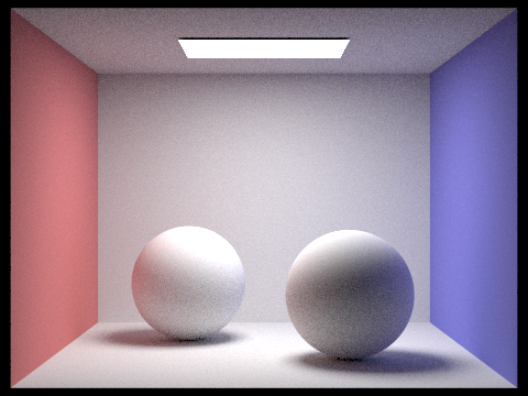 |
 |
| Low Discrepancy Sampling |  |
 |
The low discrepancy sampling produces slightly fewer aliasing artifacts and smoother gradients, particularly in areas with complex lighting.
Part 2: Surface Area Heuristic
The Surface Area Heuristic (SAH) is a method for optimizing BVH construction by minimizing the expected cost of ray-primitive intersection tests. It evaluates potential splits based on the surface area of bounding boxes and the distribution of primitives.
SAH Algorithm Implementation
The SAH cost function for a split is defined as:
Where:
- $C_{trav}$ is the cost of traversing a BVH node (set to 1.0)
- $C_{isect}$ is the cost of ray-primitive intersection (set to 1.5, optimized ratio 1:1.5)
- $SA(L)$, $SA(R)$ are surface areas of left and right bounding boxes
- $\text{TriCount}(L)$, $\text{TriCount}(R)$ are the number of triangles in left and right partitions
Algorithm Steps:
- Multi-axis evaluation: Test splits along all three coordinate axes (x, y, z)
- Bucket-based sampling: For each axis, evaluate 12 different split positions
- Cost calculation: Compute SAH cost for each split candidate
- Optimal selection: Choose the split with minimum cost
- Fallback mechanism: Use midpoint heuristic if SAH fails (e.g., zero surface area)
Implementation Details:
- Primitive sorting: Sort primitives by centroid along each axis for split evaluation
- Bounding box computation: Calculate tight bounding boxes for left and right partitions
- Degenerate split handling: Skip splits that would create empty partitions
- Cost optimization: Select split that minimizes expected ray traversal cost
Performance Comparison
Command: ./pathtracer -t 8 -s 2048 -a 64 0.05 -l 1 -m 5 -r 480 360 -f bunny.png ../dae/sky/CBbunny.dae
| Metric | Original BVH (Midpoint) | SAH-Optimized BVH |
|---|---|---|
| Construction Time | 0.0086 seconds | 0.4203 seconds |
| Rendering Time | 161.3689 seconds | 92.7042 seconds |
| Average Speed | 3.0270 million rays/sec | 5.0912 million rays/sec |
| Intersection Tests/Ray | 6.209629 | 3.525061 |
Performance Analysis
The SAH-optimized BVH demonstrates significant performance improvements over the midpoint heuristic. The dramatic reduction in intersection tests per ray demonstrates the effectiveness of SAH’s cost-based optimization. By intelligently partitioning primitives based on surface area and primitive distribution, the SAH creates more balanced trees that minimize the expected number of ray-primitive intersection tests during traversal.
Part 3: Bilateral Blurring
Bilateral filtering is an edge-preserving smoothing filter that reduces noise while maintaining sharp boundaries between different objects or regions in the rendered image. Unlike traditional Gaussian blur that treats all pixels equally, bilateral filtering considers both spatial distance and color similarity when determining filter weights.
Bilateral Filter Algorithm
The bilateral filter combines two Gaussian kernels:
- Spatial Kernel: Based on Euclidean distance between pixels
- Range Kernel: Based on color difference between pixels
The filter weight for each neighboring pixel is computed as:
Where:
- $(i,j)$ is the center pixel position
- $(k,l)$ is the neighboring pixel position
- $\sigma_s$ is the spatial standard deviation (controls spatial smoothing)
- $\sigma_r$ is the range standard deviation (controls color similarity threshold)
- $I(i,j)$ represents the color value at pixel position
Algorithm Implementation Details
Mathematical Foundation:
The bilateral filter output for pixel $(x,y)$ is computed as:
Integration with Rendering Pipeline
The bilateral filter is integrated into the rendering pipeline as a post-processing step that occurs after all path tracing computations are completed but before the final image is saved. This placement ensures that the filter operates on the final accumulated radiance values, applying noise reduction without affecting the underlying path tracing algorithm, so that the filtered result with enhanced visual quality is what gets written to the output image file.
Comparison Results
The following images demonstrate the effect of bilateral filtering on a noisy path-traced image:
| spp | Without Bilateral Filter | With Bilateral Filter |
|---|---|---|
| 16 |  |
 |
| 128 |  |
 |
The comparison shows that the bilateral filter effectively reduces noise while preserving important edges and details in the image, resulting in a cleaner and more visually appealing final render.
Benefits of Bilateral Filtering in Path Tracing
- Noise Reduction: Significantly reduces Monte Carlo noise, especially in low-sample renders
- Edge Preservation: Maintains sharp boundaries between objects and materials
- Detail Retention: Preserves fine geometric and lighting details while smoothing noise
- Visual Quality: Produces cleaner, more professional-looking final images
- Sample Efficiency: Allows for acceptable image quality with fewer samples per pixel
The bilateral filter serves as an intelligent post-processing step that enhances the final image quality by leveraging both spatial and perceptual information to selectively smooth noise while preserving important image features.
Part 4: Iterative BVH Implementation
To improve performance for large scenes, we implemented an iterative BVH system using explicit stacks instead of recursion. This addresses stack overflow issues in deep trees (>10k primitives) and improves cache locality through better memory access patterns.
Algorithm Design
The iterative approach replaces recursive function calls with explicit stack management:
- Construction: Uses
std::stack<ConstructionStackFrame>with depth-first processing while maintaining SAH optimization - Traversal: Implements stack-based
has_intersection_iterative()andintersect_iterative()methods - Automatic Selection: Chooses iterative methods for construction (>10k primitives) and traversal (>5k primitives)
Key Benefits
- Performance: Better cache locality and reduced function call overhead
- Flexibility: Manual method selection available for debugging
This optimization provides significant performance improvements for large scenes while maintaining the same intersection accuracy as the recursive implementation.
Performance Comparison
Command: ./Release/pathtracer -t 32 -s 2048 -a 64 0.05 -l 4 -m 5 -r 480 360 -f bunny.png ../dae/sky/CBbunny.dae
| Metric | Recursive BVH | Iterative BVH |
|---|---|---|
| BVH Construction Time | 0.3944 seconds | 0.3893 seconds |
| Rendering Time | 171.0142 seconds | 143.4334 seconds |
| Average Speed | 4.9297 million rays/sec | 4.9389 million rays/sec |
Analysis: The iterative BVH implementation shows an improvement in rendering time, demonstrating better cache performance and reduced function call overhead. While it performs slightly more intersection tests per ray, the overall efficiency gains from better memory access patterns result in faster rendering for complex scenes.